

That is much more difficult than it sounds. There is no observing system capable of measuring temperature, humidity, pressure and wind at every point on Earth, at every height, at exactly the same time. Instead, meteorologists work with a patchwork of information from satellites, weather stations, radiosondes, aircraft, ships, buoys and radar. These observations differ in coverage, timing and accuracy, and large parts of the atmosphere are never measured directly.
Yet a numerical weather model needs a complete three-dimensional starting state. This is the purpose of data assimilation and model initialisation. They form the bridge between observations of the present atmosphere and a simulation of its future evolution.
The same principle applies to the numerical models used by meteoblue, including its own NEMS model family. Whether a model has a grid spacing of a few kilometres or several tens of kilometres, increasing its resolution does not remove the need for accurate starting conditions. meteoblue currently operates NEMS models at several regional and global scales, while its broader forecast system also integrates output from numerous external numerical models.
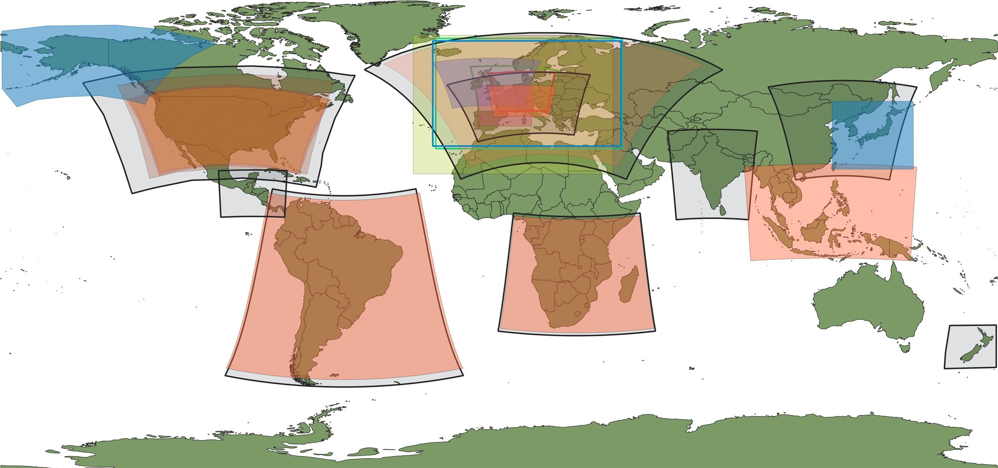
Overview of meteoblue model domains (status 2022). Global domains are not shown.
The first step is estimating the atmosphere
The state from which a numerical weather prediction model begins is known as the analysis. It is tempting to imagine the analysis as a map assembled directly from observations. In reality, it is an estimate.
Weather stations are concentrated over inhabited land areas and much sparser over oceans, deserts and polar regions. Radiosondes provide detailed vertical measurements, but only from a limited number of locations and generally only a few times per day. Aircraft provide valuable information along flight routes, while satellites offer much broader geographical coverage.
Even satellites do not simply "measure the atmosphere" in the way a thermometer measures air temperature. Many satellite instruments measure radiation reaching the sensor. From this signal, information about temperature, humidity, clouds and the surface can be inferred.
The observations come from different places and measure different parts of the atmosphere. Data assimilation combines them into one consistent picture of current conditions.
More specifically, data assimilation uses observations together with statistical and dynamical information, including a numerical model, to estimate the state of the atmosphere. In weather forecasting, that estimated state becomes the starting point of the next prediction.
The model also contributes information
Observations are only one half of the process. When a new forecast cycle begins, meteorologists already have another estimate of the current atmosphere: a short forecast from the previous model run. This is usually referred to as the background, or first guess.
Suppose the previous model run predicted that a cold front would be over eastern France at 12 UTC. New observations arriving around 12 UTC may indicate that the front is actually slightly farther east, that the air ahead of it is more humid than predicted, or that the wind behind it is stronger.
The assimilation system compares those observations with the background and determines how the atmospheric state should be adjusted. The result becomes a new analysis and the model then starts again from this revised state.
The process is cyclical: an earlier analysis produces a short-range forecast, new observations are then added to update the atmospheric state, and this revised analysis becomes the starting point for the next forecast.
This explains an important feature of operational forecasting: each forecast is connected to the one before it. A model is not rebuilt from observations alone every few hours. Information from earlier observations is carried forward by the model and updated as new data arrive. Operational assimilation systems use the previous forecast precisely because observations alone are too incomplete to describe the entire atmosphere.
Why not simply force the model to match every observation?
Because observations and models do not always describe the same scale.
For example, imagine a temperature sensor at the bottom of a narrow Alpine valley on a clear winter night. Cold air can collect near the valley floor, producing a temperature far below that on the surrounding slopes. The measurement may be perfectly correct. But a model grid cell several kilometres wide may represent an average elevation and terrain that does not fully contain that valley. Replacing the grid-cell temperature directly with the station value could actually make the model state less realistic.
Meteorologists call this problem representation error. It occurs when an observation captures very local conditions that the model grid is too coarse to reproduce. The measurement can be correct, while the model value can still be reasonable for the larger area it represents.
Representation error is an important challenge in data assimilation because detailed observations are often compared with models that cannot resolve the same level of local detail. This is especially relevant in areas with complex terrain or rapidly changing weather, such as thunderstorms, coastal zones and tropical cyclones. In these cases, the system must consider not only the observation itself, but also how well it represents the conditions at the model’s scale.
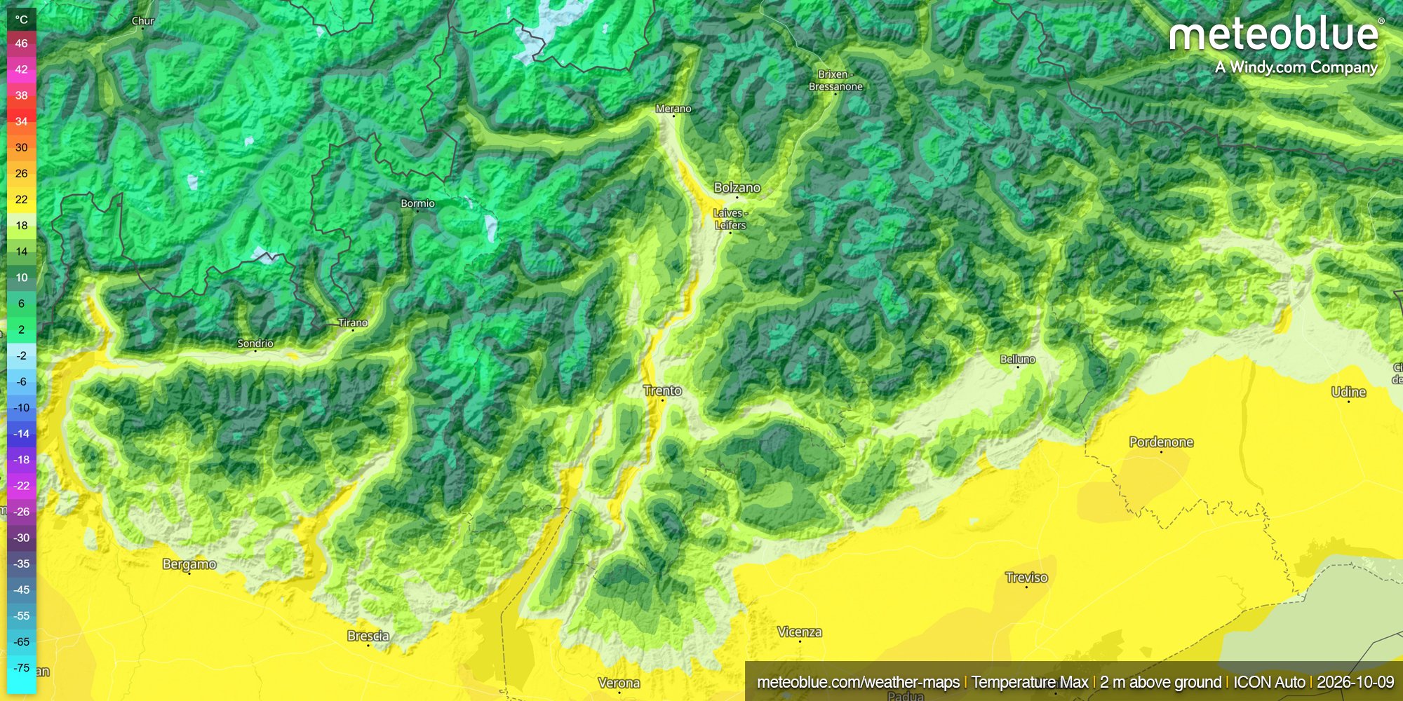
Temperature differences across Alpine valleys illustrate how local measurements can differ from the broader conditions represented by a model grid cell.
Which one should the system trust?
Neither observations nor the background forecast are assumed to be perfect. Instead, the assimilation system considers their estimated uncertainties. Where observations are considered reliable and the background is uncertain, observations can have a stronger influence. Where a measurement has larger uncertainty, or is poorly representative of the model scale, the background may retain more weight.
The process also has to account for the fact that temperature, pressure, humidity and wind are connected. A single observation can therefore affect several variables and nearby grid points. This helps keep the model atmosphere physically consistent, rather than treating each measurement separately. Determining how these atmospheric variables influence one another is one of the most sophisticated parts of numerical weather prediction.
Observations are collected at different times
Observations used to build an analysis are not all taken at the same moment. A weather balloon, aircraft report and satellite overpass may be separated by several hours, while the atmosphere continues to evolve.
One way to account for this is four-dimensional variational data assimilation (4D-Var), which considers longitude, latitude, height and time. Instead of fitting observations to a single snapshot, it looks for a starting state that stays consistent with observations collected throughout the assimilation period.
Ensemble methods take a different approach, using a set of slightly different model states to estimate uncertainty and relationships between forecast errors. Modern forecasting systems increasingly combine variational and ensemble techniques.
Initialisation is not limited to the atmosphere
Once an atmospheric analysis exists, there is still more work to do. A weather model also needs a realistic description of the surface beneath the atmosphere. Soil moisture, soil temperature, snow cover and snow temperature can influence the forecast from its first hours.
Soil moisture is especially important, because it affects how incoming energy is divided between heating the ground and evaporating water. A model that starts with soil that is too dry may allow the land surface to heat too strongly, changing near-surface temperature, humidity and the development of the boundary layer.
Snow alters both the surface energy balance and exchanges of heat and moisture. Changes in the initial soil-moisture and snow state can affect not only surface forecasts, but also the atmosphere above them.
The starting state must also be dynamically consistent. If assimilation introduces abrupt adjustments to pressure, wind or temperature, the model may respond with unrealistic oscillations as it tries to regain balance. That is why some systems introduce analysis corrections gradually. One method, known as incremental analysis updating, was developed to reduce these initial adjustment problems and the associated "spin-up" of model processes such as precipitation.
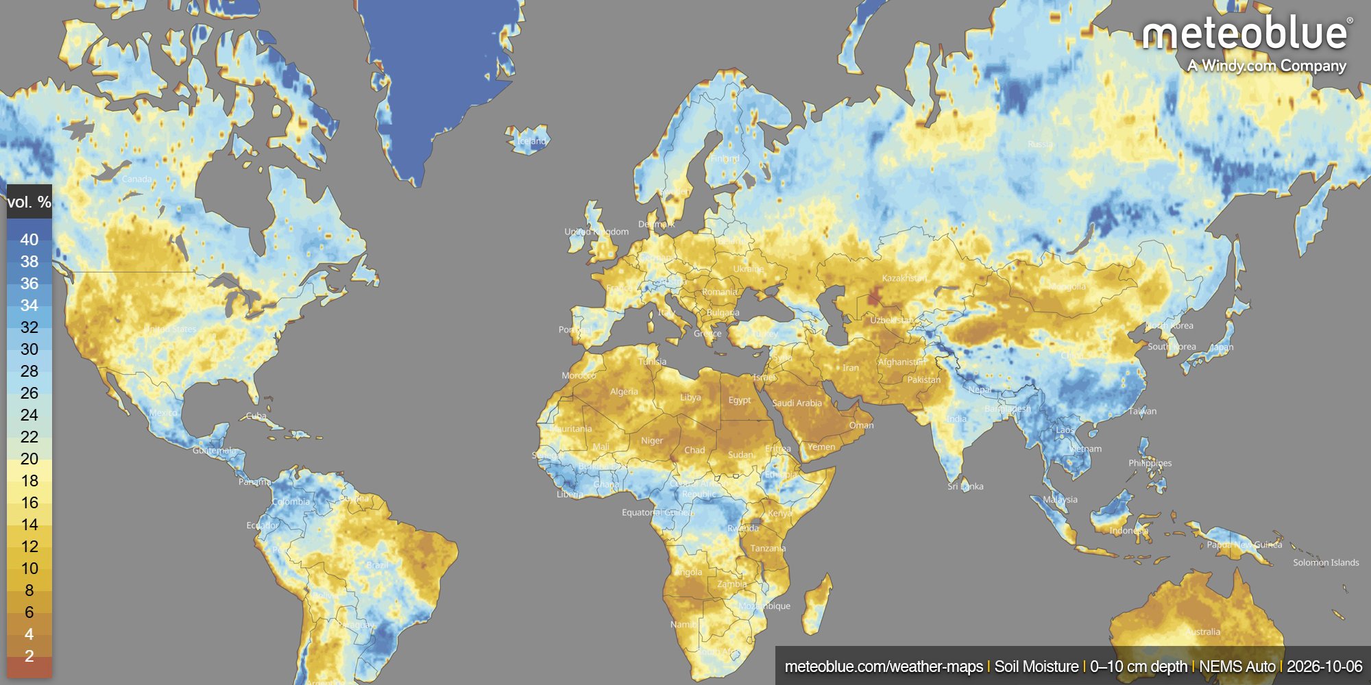
Soil moisture is an important part of model initialisation, influencing surface heating, evaporation and the atmosphere above.
Where mLM enters the forecast chain
Data assimilation focuses on the starting state of the atmosphere. Once the numerical models have run, another question becomes important: how well does their output represent conditions at a specific location?
Different models have different resolutions, physics and update cycles, so their performance can vary by place and weather situation. Post-processing helps account for these differences before the forecast reaches the user.
The meteoblue Learning MultiModel (mLM) combines forecasts from several numerical weather models using machine-learning methods and recent performance data. The model mix can change as new forecasts and observations become available. For suitable weather stations, mLM can also use the relationship between past forecasts and measurements to adapt predictions to local conditions.
This is different from data assimilation: data assimilation improves the atmospheric state used to start the simulation, while mLM works with the forecasts produced afterwards, combining and refining their output.
Why forecasts change from one update to the next
Forecasts can change between updates even when the underlying weather models have not changed. New satellite, radiosonde or aircraft observations may slightly shift the analysed position of a trough, the moisture ahead of a front or the strength of the jet stream. Small adjustments like these can influence how weather systems develop several days later.
As new model runs become available, the forecast system also reassesses their performance. Each update can therefore begin from slightly different atmospheric conditions and use a different mix of model guidance.
Uncertainty still remains. Observations are incomplete, measurements and models have limitations, and small errors in the initial state can grow with time. This makes accurate starting conditions essential, even though no forecast can be perfect.
Before a rainfall map, temperature curve or weather icon appears, observations have already been collected, checked and combined with earlier forecasts to build the best possible picture of the atmosphere.
That is where every forecast begins.
Want to continue the discussion? Visit the meteoblue Community Forum to ask questions, share ideas and exchange perspectives on weather and forecasting with other members of the community.


